I haven’t posted for a while because I’ve been a bit stuck with this interesting, yet frustrating MOOC on Coursera. According to the marking system, I’ve passed, so I wanted to share what I learned about how statistics help drones (or any intelligent robot) navigate. Check out my code to generate the below simulation.

Uncertainty

If you are driving a car, the speedometer will tell you that you’re going at 50 mph. You will know that you’re going at 50 and not 55, but you probably won’t  be able to tell if you’re going at 49.96 or 50.05. This may be because the needle is too thick or because there is a tiny imbalance in some part of the machinery connecting the axle to the gauge. Fortunately, we don’t care whether we’re going at 49.96 or 50.05 mph because it makes no material difference to how we drive.

Whilst humans are usually very certain about where they are, where their nose is pointing and how many steps they need to climb, it turns out uncertainty is a massive problem for autonomous systems like robots.

Imagine a missile travelling at 2.8 km per second needing to intercept a 1m wide asteroid on a collision course with a new space station – if the missile is travelling 500km to hit its target, it needs to be controlled incredibly accurately to make sure all the small imperfections on the way don’t take it off track. It may be that the accelerometers on board have a manufacturing tolerance that means their readings can be out by 5%. What to do? How do we direct it if we’re not sure how fast it is?

Statistics

Disclaimer: I used to hate statistics at school and my early working days because we went straight into the equations without talking about the essence. Since dabbling in machine learning and robotics, I now appreciate the need.

For example: If I know exactly what the market will be tomorrow, I can take only one action to plan for it precisely and optimally, but if I don’t, I need to consider the different scenarios and either plan for the most likely one(s), or ideally all of them.

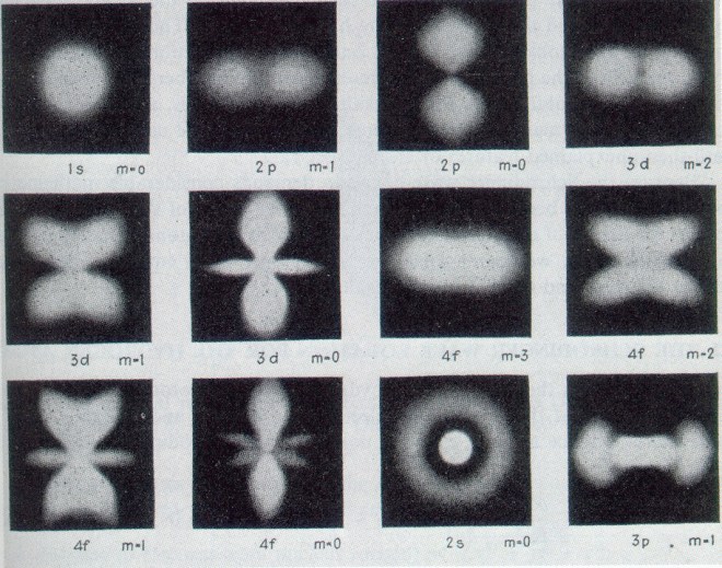
Similarly, for a given atom energy level, an electron “cloud” is a representation of all possible locations of an electron around its nucleus, weighted by probability. The electron is so small, fast and damn spooky that it makes more sense to represent and use all its possible positions for analysis, rather than keep track of the crazy particle.

Statistics gives us a way to manipulate the entire distribution, rather than individual certain events (samples). If we have a process that takes a variable through a large number of steps, the variable becomes the distribution – the collection of all  outcomes weighted by probability – instead of a single discrete observation.

We typically end up with better predictions by carrying the uncertainty through the process; one way to think about this is that after a large number of random events the “noise” typically averages out.

Another key idea in statistics is inference, for example in Bayes’ Rule, where we can work backwards; from a series of observations we can infer the most likely probability distribution that they were observed from. It’s quite important to read up on this before attempting the MOOC mentioned in the next section.

Kalman Filter and “Sensor Fusion”

Imagine chasing a friend through a thick forest. You hear a shuffle, you turn towards it. You catch a blur, your eyes focus. You smell his fear… okay, maybe a bit weird, but you get the idea – the information you have about your friend’s location increases as you take more independent measurements. Or, statistically: your estimate of your friend’s location is less uncertain (has less variance) if you use both your eyes and ears, than if you use only one of them independently. This is sensor fusion – kinda.

In this MOOC you can learn about one way of implementing a sensor fusion algorithm for a robot that decides where it is using a combination of its last position, the reading from its wheel transducers (how far it thinks it moved) and inertial sensor information – all of these variables carry uncertainty (noise) which is assumed to be Gaussian, making it easier for us to combine them in closed form.

Localisation Using a Particle Filter

Imagine we fly our robot into a dark cave on a rescue mission. GPS doesn’t work in the depths of the cave. Still the robot needs to be able to navigate; it needs to map the inside walls, avoid them and report its position. The robot needs to be light so it has the bare minimum of sensors on it; an inertial reference unit (IRU) to measure its acceleration in its own body-centered frame of reference, a light detection and ranging system (LIDAR) to measure the distance to walls and obstacles, some simple on-board logic and a long wave radio to communicate coordinates and acceleration back to the controller.

From its first position it returns the part of the cave it can see using LIDAR, with some uncertainty. It moves a tiny bit and returns an updated map reading from the LIDAR – the parts of the cave which agree in both LIDAR readings become more certain, starting to look like more solid walls.

The IRU should help us keep track of the robot’s acceleration, but it will not be perfect because of its resolution and noise during transmission. This inaccuracy builds up, especially if we are integrating acceleration twice to get position. Here is where we rely on the previous LIDAR map readings to help us pinpoint location, or localise.

The Localisation Journey

Suppose the IRU tells us we have moved by a certain amount from our last position to position A. Not trusting it completely, we instead assume our next location is a probability distribution (like the electron cloud!) which A belongs in. This way we can use statistics to work with uncertainty and help us average out noise along the journey.

We have to use some other information to help us prove which distribution we are most likely to be in – we can use the map! It’s like when somebody gives you directions then calls you when you’re nearby and asks “what can you see?”

The localisation problem then becomes: given what we can see in the vicinity of position A, what is the most likely probability distribution of our location? This is an application of Bayes’ rule.

This is an area of active research and guesswork – which probability distributions do we assume we are in? The Guassian is a common one to use because it is easy to manipulate with closed form math. To make the computation much faster we randomly pick a few positions (particles) to test from each candidate distribution. What follows is something like this:

# You are given the latest and best-known map 
# You are given a best estimate of your previous position (Distribution Z)
# You are given a new set of LIDAR readings and IRU measurement
# Where are you?

Start
Try DistributionA 
 Project a number of particles from Z using IRU plus some perturbation
 For each particle
     Record how well the LIDAR readings correspond to the map
 End
 Does the distribution of LIDAR scores for the particles correspond 
 to DistributionA? [True or False]
 If True
    Select Distribution A as distribution of new position
    Update Distribution Z as Distribution A
 End and Exit
 If False
    Go back to Start
 End

In reality a huge amount of tuning, optimization and tweaking is needed to get something that works given the dynamics of the vehicle and the quality of the sensors. For a land-rover buggy in a given map you can check out the MOOC sandbox example and my code here.