This is a quick theoretical guide on controlling linear dynamic systems, with practical advice for DIY Drone Controllers wanting to implement their own code. If you are an undergraduate engineer, graduate STEM or a tinkerer with a basic understanding of differential equations, this should make sense and hopefully help you!

What is closed-loop control?
Suppose you want to sprint to a wall in the shortest time – do you run at full pace then come to a sudden stop? If you try to, most humans will hurt themselves, and either brake too late and hit the wall, or end up short. Instead, we apply a varying level of speed to our legs. But how much nerve impulse do we send to each leg muscle, and how often?
We use our eyes do determine position and speed, but we also use our amazing ears to determine speed and acceleration! During our sprint, we frequently measure how close we are to the wall, and how quickly we’re moving. We gradually adjust the demand on our muscles, and repeat that in a “closed loop” until the error (distance from the wall) is zero. Controlling vehicles has many parallels.
A hovering drone without a controller is dynamically unstable, like an upside down pendulum. If you tip it slightly, it will wobble and go all over the place. It needs a constant correction of orientation to stay upright, or move anywhere, and that needs to be automated.

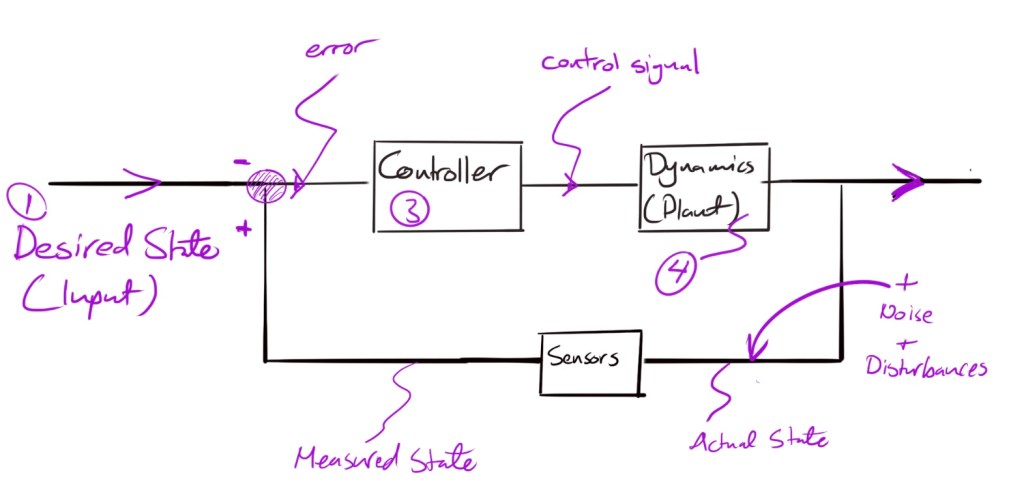
Control theory is one of most beautiful things I learned in undergraduate engineering. It looks to give mathematical answers to the question: what should I do, given where I am, and where I want to be? That includes staying still! Most control systems can be simplified into the block diagram below:

Purple lines are signals. Black Boxes are functions or processes — (called transfer functions in the frequency domain). We can design the controller, but the Dynamics of the Plant (thing to be controlled, e.g. power plant or drone) are given to us by nature, e.g. mass, length and outside our control.
In this blog, we examine each of the the elements 1-4 of a simplified closed loop controller for a drone design, along with practical advice on each, to help implement your own.
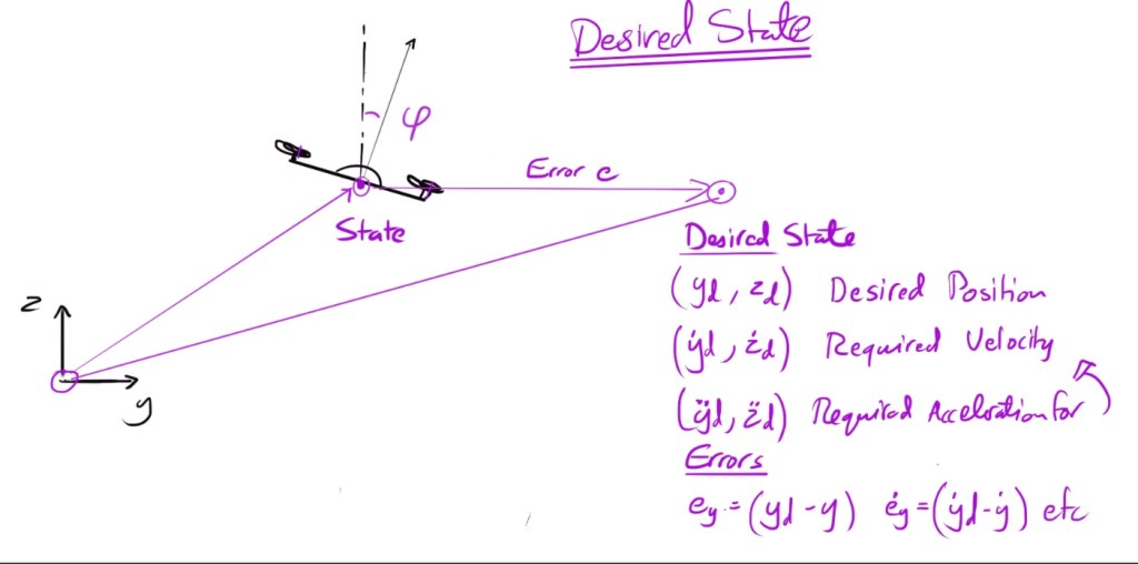
To illustrate the key principles we will assume a that our “Plant” is a 2D drone in a flat plane with its x-axis pointing into the page. This greatly simplifies the Dynamics. Here is my own python code for a simple 2D interactive controller where I use the assumptions below and the variables and equations in purple.

Controlling a 3D drone is very similar to a 2D one, although the dynamics module becomes more complex, and we need to transform between the drone frame of reference to the inertial. A good place to learn these for 3D is the UPenn Aerial Robotics Online Course, to which I’ll refer often. I credit the Upenn course also with most of my learning in this area (thank you!). If you really want to fast forward you can see my code for a non-linear 3D controller here.
1. Getting the Desired State
In Theory
Remember that telling the drone to stay still is a desired state (and needs to be controlled against e.g. wind gusts etc…). Otherwise, moving is a series of desired states:
For a human-piloted drone, the pilot will have a route in mind. Using a joystick or some other device, we tell the drone controller what position it needs to be in – the desired state. A joystick can (in theory) communicate information on desired position, velocity and acceleration by moving the joystick knob close or far, abruptly or slowly.
An drone on autopilot will normally be given way-point coordinates from a controller based on a desired path. But does it go between each of them in a straight line? That’s the subject of route planning.
In Practice for a Drone
Suppose you want the drone to touch a number of coordinates. There are an infinite number of paths it can take between them. You can plan a path that maximises speed, minimises acceleratrion, or even minimises something called “Jerk” which is the rate of change of acceleration
Minimum jerk trajectories are popular as they minimize the stress on drone components by avoid abrupt, tight turns, keeping its movement smooth.
Route planning generates a desired trajectory, which is a series of desired states that vary with time. Using the desired coordinates as solution points, you can find (for example) a minimum jerk trajectory by finding a curve that smoothly fits the desired coordinates.
Here’s an example of a minimum jerk trajectory in 3D that I implemented in MATLAB in the UPenn Course, along with an explanation of why it needs to be a polynomial of the 7th power of time.
2. Getting the Actual State
How do we know the current state? Namely, where is the drone, which direction its pointing (attitude) or how quickly is it moving? This also depends on whether you’re flying a real drone or simulating one using a computer model.
If you are piloting a real drone, you should be able to see it. That’s a good estimate for position, but maybe not acceleration. If the drone is beyond visual range, it will need to communicate back to you its position, acceleration and attitude. You could even get a real-time feed from some camera mounted to it, but that can be heavy, energy intensive and slow.
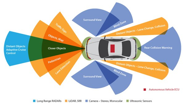
You could instead get small measurements from sensors like GPS (position), LIDAR or ultrasound (distance to obstacles) accelerators (linear acceleration) and gyroscopes (rate of rotation). The latter two don’t rely on vision so are called Inertial Reference Units (IRU) in most vehicles. Remember: the main things we need for the state are the position and attitude, and their rate of change.
In Practice for a Drone
Unfortunately, no sensor is 100% accurate – they all have a minimum resolution. Moreover, getting a sensor reading from source to computer involves a number of electronic circuits and analogue-digital signal conversions — these can introduce noise or even errors.
The IRUs only give us acceleration, so we need to integrate that over time to get position — this risks compounding errors.
All of this means we are never controlling the desired state against the actual state, but rather the measured state. There are a number of ways to get around this in practice:
- Redundancy Using a number of independent sensors to measure the same variable, both for backups and to increase confidence.
- Statistical Noise Reduction Accounting for noise by statistical methods like Kalman Filters that compare the predicted next state with what the sensors actually read. By combining the noise distribution of both, the uncertainty is reduced … (assuming the noise is truly random). I wrote an article previously that demonstrates a simple Kalman filter for a drone with both inertial measurements and LIDAR readings against a known map. It also discusses sensor fusion more broadly.

- Modelling the noise Accounting for sensor noise in the design of your control system, by adding a transfer function between the actual state and measured state.
3. Designing the Controller
Now that we have the error between current and desired state…
In Theory
The Controller takes the error between desired and current state as an input, and outputs a control signal (e.g. electrical current) to the plant (the thing being controlled, e.g. a motor). How does the controller relate the output signal to the error? There are normally three ways to do this:
- Proportional control relates the output signal to the error through a proportionality constant called the proportional gain Kp so that Output = Kp times the position error. This is the simplest and most commonly used control gain.
- Derivative control uses another proportionality constant Kd and calculates the output signal as a multiple of this times the error in the first derivative (i.e. speed) of the state. This can help in damping the response if we want a high proportional gain
- Integral control calculates the output control signal as a function of time and the total error up to that point (the integral of the error). This helps counter any offsets or persistent bias in the sensors or plant, even after the (instantaneous) error goes to zero. We won’t use integral control for this Drone.
The Proportional, Derivative and Integral elements can be combined in a variety of ways to form the family of PID controllers. A correctly designed PID control system can be mathematically proven to drive the error exponentially to zero in a way that is stable.
Control system design, and stability, is an engineering degree in itself and too wide to describe in this blog or website. Below are some of the things to consider for a drone.
In Practice for a Drone
In the case of the drone the motors point vertically. Controlling the vertical height is a straightforward relationship with the motor speed and is nearly linear. So our diagram for a simple 2-box control system would actually work. But controlling the horizontal motion is more complicated because there are no horizontal facing motors (the drone is not fully actuated).
We first need the drone to tilt just a little so that there is a component of its force in the x or y directions. Tilting introduces non-linearity (see dynamics) because of the Sin and Cos functions, but it also means there is a loop within a loop in our control system, each with separate gains. First we need to decide how much to tilt by, then we need to order the motors to change speeds to generate the moment.


The controller I have design is a PD controller so you will only see Kp and Kd terms above, with a further subscript for y, z, or psi (tilt) depending on the axis.
Tuning the gains (choosing their value) is also a bit of an art. There are some simple heuristics like the Ziegler-Nichols method that can help you get there without too much pain, as trial and error can seem endless.
I’m sure gradient descent like in machine learning could be used as an automatic tool to tune controller gains, but I have not looked into it. [If we are to believe this UC Berkley Machine Learning Researcher, few people have made the link until recently!]
During most of my control engineering degree, we assumed the systems we were controlling were Linear and Time Invariant (LTI). We indeed assume this for our drone, although in reality no system is LTI, so the below reasons mean your simulation will never match reality perfectly:
Linear dynamic systems obey the superposition principle. So for example if you run twice the current through a resistor, it generates twice the voltage. For our drone, this is not really the case because of the horizontal motion requiring a tilt as an intermediate step – the horizontal force is actually trigonometric in angle, and not linear (and Sin(A)+Sin(B) =/= Sin (A+B)!).
We use the small angle approximation that Sin(A) ~ A but that limits our drone to fairly gentle maneuvers where it doesn’t tilt too much. For an example of a non-linear controller, have a look at this MATLAB example from the UPenn code — this allows a wilder drone but may be more difficult to prove stability.
Linear controller gains also shouldn’t depend on the state, so twice the error should causes twice the output signal whatever the state. In reality though, our motor thrust will not be linearly proportional to the electric current, as prop blades aerodynamics vary with tilt. For small drones this is negligible at shallow angles, but it’s a different story in helicopters.
Time Invariant systems assume that the Dynamics (and hence Controller) functions don’t change with time, so they are just one equation we hard-wire at the beginning and that they work for all possible states of the Drone.
In reality, aircraft burn fuel and their center of gravity shifts as they fly, so their dynamics do change and so must the controller to ensure a smooth experience for passengers. The drone dynamics are fairly time invariant (although when the battery gets low, the responsiveness of the motors may suffer).
4. Modelling the Dynamics
After applying the forces to our Drone… what happens?
In Theory
In the Dynamics module of the control system, we take the forces acting on the body, and calculate the resulting motion based on the system’s equations of motion.
It is not essential to know or calculate the equations of motion when designing controllers for complex systems. Many times it’s impossible, so we just measure the output of the system and take that as the next current state.
For LTI systems we can reverse engineer the equations of motion (in a sense) by measuring the plant’s impulse response; that is, its vibration frequency and decay rate resulting from a tap, like a tuning fork!

Most engineering systems can be reasonably simplified into LTI systems obeying linear second-order differential equation (analogous to the mass–spring-damper system, or damped harmonic oscillator) and their impulse response characterizes them fully. (No real world system is truly LTI though).
However, if we want to simulate the drone’s motion in our case, we need to know it’s equations of motion, or at least estimate them from first principles. This is especially important if we want to simulate the drone responding to unpredictable inputs like a human controller.
In Practice for a Drone
In the below image we show the most basic representations of Newton’s F=ma equations of motion for our drone, taken instantaneously. For a 2D system, these are actually sufficient to model the dynamics.
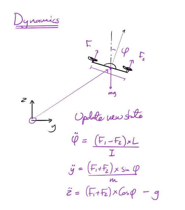
This is a linear map between the external forces, orientation, weight of the drone, and its resultant acceleration. To simulate and plot the trajectory of the drone we have two options:
- Real Time Simulation: solve the equations of motion instantaneously at short time intervals, then “plot as we go”, then solve again after the drone has moved through a few milliseconds, and so on.
- Replay Simulation solve the equations of motion for given interval (example 0-10 seconds), store the trajectory and then replay the whole thing in “simulated” real-time.
Take a look at my python code for both here.
In both cases for a 2D drone, by “solving” the equations of motion we are evaluating the acceleration then estimating the resultant velocity (and hence position) at small time intervals using discrete integration — which is a Taylor Series approximation.
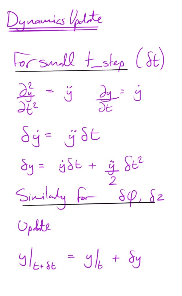
In 3D, the equations of motion become non-linear: the acceleration doesn’t depend just come from external forces, but from rotating simultaneously around two or more body-fixed axes (gyroscopic effects), we can’t quite use the method above. A numerical solver like ODE45 is used to find a solution for the acceleration and velocity at the same time, that is within an acceptable margin of error (tolerance) — again at discrete time steps.
Replay simulations won’t work well for a user-controlled simulation or game, however for reasons discussed in section 5 (time) they are smoother. Real-Time Simulation is tricky, because we want the the time intervals to be small enough to accurately evaluate the speed and velocity using Taylor series, but we don’t want to perform so many complex calculations between each frame update to the screen…
5. Time … and the real world
In Theory
To bring everything together, the controller is constantly looping through these four steps (or 3 if you are going for a replay at the end)
1 Get desired state
2 Measure current state
3 Calculate control signal
4 Estimate next state using Dynamics and ideally plot it (Not essential, unless you want to simulate or model the system).
In Practice for a Drone
Using timers in my code and a 5 year old i5 processor, I think the reality looks a little more like this.
1 Get desired next state by regularly checking the pilot remote controls, calculating any pre-programmed trajectories (10s of microseconds)
2 Estimate the current state by polling sensors at a fixed rate, converting visual information into location information, estimate speeds by integrating accelerator data (10s or 100s of microseconds)
3 Calculate control signal (a few microseconds for a linear controller, 10s or more for a non-linear one) and issue the motor commands to the power unit (microseconds-milliseconds)
4 Estimate the next state using the dynamics, or solve the complete simulation by solving the differential equations of motion (10s of microseconds per second of simulation)
And/or wait for the control signal to turn into motor current to turn into a rotating fan (inertia) to turn into thrust (fluid dynamics).
And/or plot or render your drone position and attitude (10s of microseconds at best in Matplotlib)
What this means is that the simulation time is not equal to the real passage of time – by the time the solver and plotter has got to the 5th second of the real simulation, it may have expended (for example) 5.2 seconds of computing time – the 0.2 seconds being computing time to run through the 4 steps above – let’s call this “The Matrix delay”
The “Matrix delay” could be reduced by a faster computer, but much depends on your CPU clock speed, and whether you can get the CPU to entirely devote itself to the above process. A Raspberry Pi for example runs python within Linux and doesn’t guarantee how many RAM or clock cycles your python programme gets. To control that more tightly you could use a dedicated computer, which could even be a small one like an Arduino that either loops a single programme, or turns off.
Also, compiled programming languages like C++ run faster than interpreted languages like Python, so any serious realtime application needs to be written in the former. C++ also ringfences memory so you have a better chance of dedicated processing power.
Finally, live plotting graphics is time consuming and I don’t understand it well enough just yet. What I do know is python’s standard plotter Matplotlib is not particularly fast. It took me a while to find ways of getting it to plot the output of a script while in parallel listening to keyboard and joystick inputs. Here are a few ways to do that (includes link to a wiring diagram for a RaspberryPi joystick controller input).
Most professional aircraft control systems and robots have dedicated computers running solely one function. For my first DIY drone though, I’m going to see how far I can get with using a Raspberry Pi. Stay tuned!
